Unveiling the Power of Completely Randomized Design (CRD) in Crop Science Experiments

In the vast expanse of crop science, where precision and reliability are paramount, the choice of experimental design plays a pivotal role in unlocking the secrets of optimal crop growth. Among the arsenal of experimental methodologies, the Completely Randomized Design (CRD) emerges as a beacon of simplicity and statistical robustness. In this blog, we embark on a journey into the realm of CRD, unraveling its principles, applications, and the advantages it brings to the forefront of crop science research.

Understanding CRD: A Statistical Marvel

What is Completely Randomized Design (CRD)?

CRD is a statistical method that serves as a robust tool for comparing the effects of different treatments on a single factor within crop experiments. It operates on the principle of randomness, ensuring that each experimental unit has an equal and unbiased chance of receiving any treatment. This randomization process is pivotal, eradicating potential biases and attributing observed crop responses solely to the applied treatments.

When to Use CRD:

CRD finds its niche in situations where experimental units are relatively homogenous, and there are no discernible patterns of variability within the experimental area. It is particularly valuable in small-scale or preliminary studies, where the primary objective is to gather initial data, identify trends, and pave the way for more intricate experimental designs.

Conducting a CRD Experiment: Steps Unveiled

Define the Research Question and Identify Treatments:
- Begin by articulating the research question you aim to answer. Identify the treatments relevant to the research question, laying the groundwork for a focused and purposeful experiment.
Prepare the Experimental Area:
- Select a uniform experimental site, ensuring consistency in soil conditions, topography, and other relevant factors. Divide the area into individual experimental units of equal size to maintain comparability.
Label the Experimental Units:
- Assign unique identifiers to each experimental unit. This step facilitates tracking and systematic data recording throughout the experiment.
Randomly Assign Treatments:
- Utilize a random number generator or a randomizing device to assign treatments to experimental units. This step ensures an unbiased distribution of treatments, a key feature of CRD.
Apply Treatments:
- Implement the assigned treatments to the respective experimental units. Keep accurate records of application dates, quantities, and methods to maintain precision in data collection.
Collect Data:
- Regularly monitor the experimental units, collecting pertinent data on crop growth, yield, and any other relevant parameters. Consistent and systematic data collection is crucial for the success of the experiment.
Analyze the Data:
- Employ appropriate statistical methods to analyze the collected data. Determine whether there are significant differences in crop responses among the different treatment groups, providing valuable insights into the effectiveness of each treatment.

Advantages of CRD: Unraveling Simplicity and Robustness

Simplicity: CRD’s conceptual straightforwardness and ease of implementation make it accessible to researchers of varying experience levels. Its simplicity is a virtue that expedites the experimental process without compromising reliability.

Flexibility: CRD’s adaptability shines through, accommodating a wide range of experimental setups. This flexibility allows researchers to explore various factors and treatment combinations, offering versatility in experimental design.

Statistical Efficiency: By providing a statistically sound basis for comparing treatments, CRD ensures that conclusions drawn from the experiment are valid and reliable. This statistical efficiency is critical for making informed decisions based on experimental outcomes.

Wide Applicability: CRD’s versatility extends across different crop types and experimental environments, making it a valuable tool for crop scientists working in diverse agricultural landscapes.

Applications of CRD in Crop Science: Navigating Agricultural Frontiers

CRD has found widespread application in various facets of crop science research, including:

Evaluating Fertilizer Effectiveness:
- CRD is instrumental in assessing the impact of different fertilizer rates and application methods on crop yield and nutrient utilization efficiency.
Comparing Crop Varieties:
- Researchers leverage CRD to compare the performance of various crop varieties under different environmental conditions, aiding in the selection of optimal cultivars.
Optimizing Irrigation Practices:
- CRD facilitates investigations into the effects of different irrigation regimes on crop yield and water use efficiency, contributing to water conservation efforts.
Exploring Tillage Practices:
- Researchers delve into the effects of different tillage practices on soil health and crop productivity, using CRD as a systematic approach to experimentation.

In essence, CRD serves as a linchpin for crop scientists, offering a systematic and statistically sound approach to experimentation. Through its application, researchers generate reliable data that not only informs agricultural practices but also contributes to the broader understanding of crop dynamics, fostering innovation and sustainability in the realm of crop science.

The fields of green are not just a canvas for growth; they are a stage for scientific inquiry, and CRD takes center stage in unraveling the intricacies of crop science.

Mastering Completely Randomized Design (CRD) Analysis with AgroR package

Conducting a thorough analysis of Completely Randomized Design (CRD) experiments in crop science can be a powerful tool for understanding treatment effects. Utilizing the AgroR package in R, you can navigate through the analysis seamlessly. Follow these steps to unlock meaningful insights from your CRD data:

Step 1: Set the Stage with AgroR

Install and Load the AgroR Package

Begin by installing the AgroR package using the following R command:

install.packages("AgroR")

After installation, load the package into your R session with:

library(AgroR)

Step 2: Prepare Your Data for Analysis

Ensure your CRD data is well-organized in a data frame with the following structure:

Each row represents an experimental unit.
The first column contains treatment assignments (e.g., “Treatment 1”, “Treatment 2”, etc.).
Subsequent columns hold measured values for each experimental unit and response variable (e.g., yield, plant height).

Step 3: Unveil Patterns with Analysis of Variance (ANOVA)

Utilize the DIC function to perform ANOVA on your CRD data:

data(pomegranate)

with(pomegranate, DIC(trat, WL, ylab = "Weight loss (%)")) # tukey


-----------------------------------------------------------------
Normality of errors
-----------------------------------------------------------------
                         Method Statistic   p.value
 Shapiro-Wilk normality test(W) 0.9448293 0.2087967

As the calculated p-value is greater than the 5% significance level, hypothesis H0 is not rejected. Therefore, errors can be considered normal


-----------------------------------------------------------------
Homogeneity of Variances
-----------------------------------------------------------------
                              Method Statistic   p.value
 Bartlett test(Bartlett's K-squared)  8.568274 0.1275737

As the calculated p-value is greater than the 5% significance level,hypothesis H0 is not rejected. Therefore, the variances can be considered homogeneous


-----------------------------------------------------------------
Independence from errors
-----------------------------------------------------------------
                 Method Statistic   p.value
 Durbin-Watson test(DW)  2.104821 0.1924474

As the calculated p-value is greater than the 5% significance level, hypothesis H0 is not rejected. Therefore, errors can be considered independent


-----------------------------------------------------------------
Additional Information
-----------------------------------------------------------------

CV (%) =  10.84
MStrat/MST =  0.92
Mean =  2.2596
Median =  2.225
Possible outliers =  No discrepant point

-----------------------------------------------------------------
Analysis of Variance
-----------------------------------------------------------------
          Df   Sum Sq    Mean.Sq  F value        Pr(F)
Treatment  5 3.692121 0.73842417 12.31191 2.723541e-05
Residuals 18 1.079575 0.05997639

As the calculated p-value, it is less than the 5% significance level.The hypothesis H0 of equality of means is rejected. Therefore, at least two treatments differ



-----------------------------------------------------------------
Multiple Comparison Test: Tukey HSD
-----------------------------------------------------------------
     resp groups
T5 2.6375      a
T4 2.6200      a
T3 2.6175      a
T6 2.1625     ab
T1 1.8425      b
T2 1.6775      b

use mcomp to multiple comparison test (Tukey (default), LSD, Scott-Knott and Duncan)

with(pomegranate, DIC(trat, WL, mcomp = "duncan", ylab = "Weight loss (%)"))


-----------------------------------------------------------------
Normality of errors
-----------------------------------------------------------------
                         Method Statistic   p.value
 Shapiro-Wilk normality test(W) 0.9448293 0.2087967

As the calculated p-value is greater than the 5% significance level, hypothesis H0 is not rejected. Therefore, errors can be considered normal


-----------------------------------------------------------------
Homogeneity of Variances
-----------------------------------------------------------------
                              Method Statistic   p.value
 Bartlett test(Bartlett's K-squared)  8.568274 0.1275737

As the calculated p-value is greater than the 5% significance level,hypothesis H0 is not rejected. Therefore, the variances can be considered homogeneous


-----------------------------------------------------------------
Independence from errors
-----------------------------------------------------------------
                 Method Statistic   p.value
 Durbin-Watson test(DW)  2.104821 0.1924474

As the calculated p-value is greater than the 5% significance level, hypothesis H0 is not rejected. Therefore, errors can be considered independent


-----------------------------------------------------------------
Additional Information
-----------------------------------------------------------------

CV (%) =  10.84
MStrat/MST =  0.92
Mean =  2.2596
Median =  2.225
Possible outliers =  No discrepant point

-----------------------------------------------------------------
Analysis of Variance
-----------------------------------------------------------------
          Df   Sum Sq    Mean.Sq  F value        Pr(F)
Treatment  5 3.692121 0.73842417 12.31191 2.723541e-05
Residuals 18 1.079575 0.05997639

As the calculated p-value, it is less than the 5% significance level.The hypothesis H0 of equality of means is rejected. Therefore, at least two treatments differ



-----------------------------------------------------------------
Multiple Comparison Test: Duncan
-----------------------------------------------------------------
     resp groups
T5 2.6375      a
T4 2.6200      a
T3 2.6175      a
T6 2.1625      b
T1 1.8425     bc
T2 1.6775      c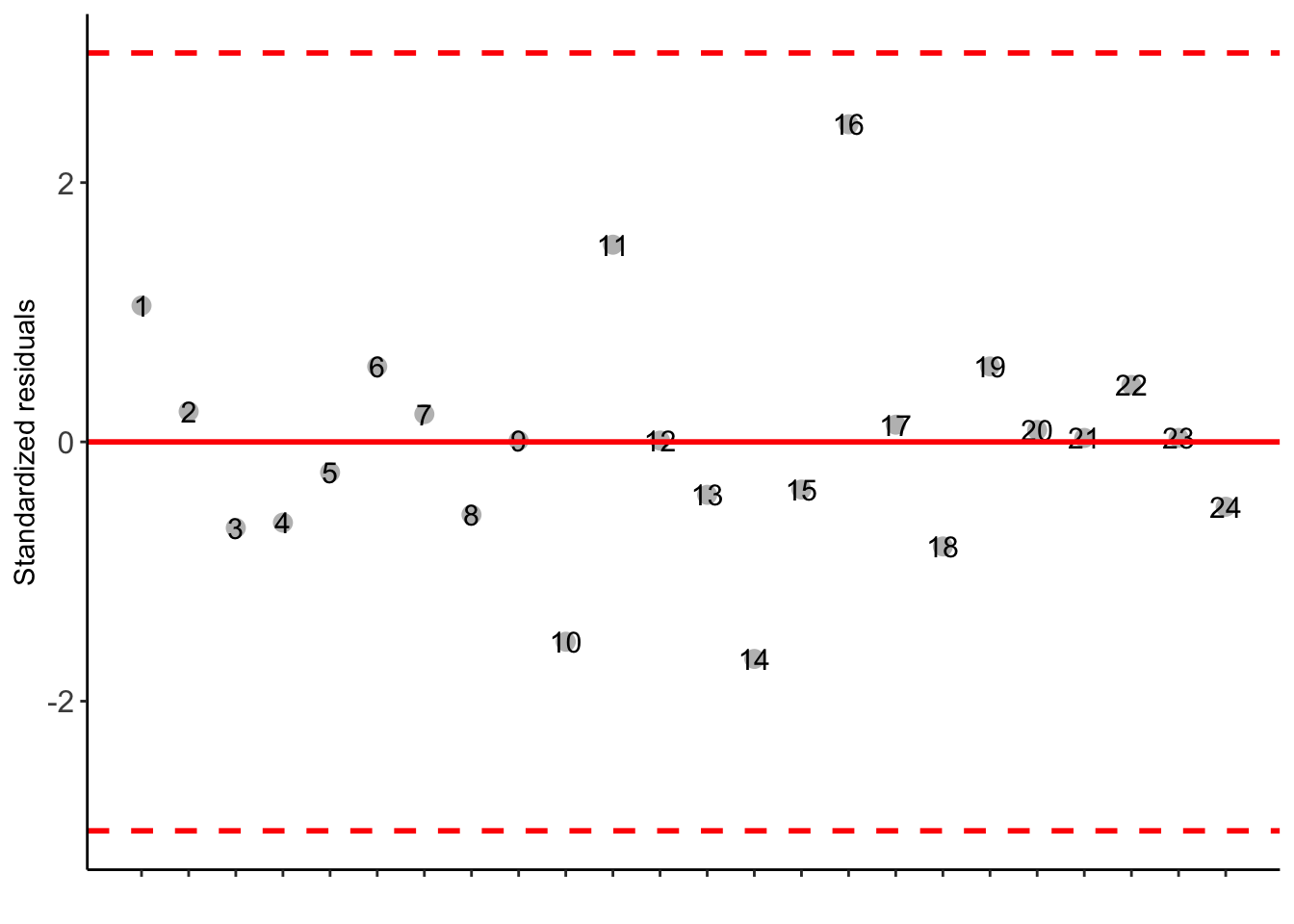

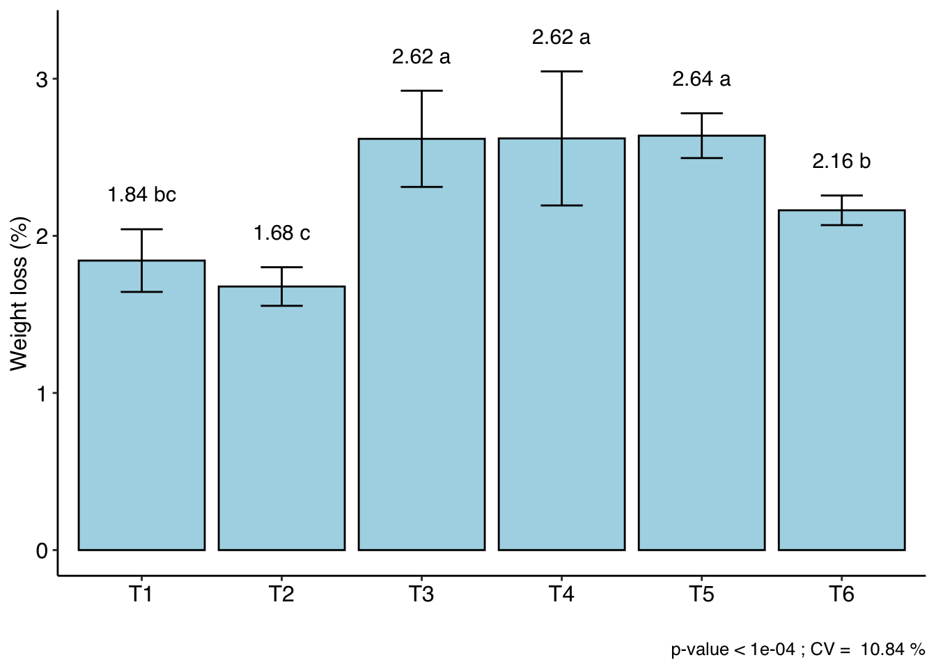
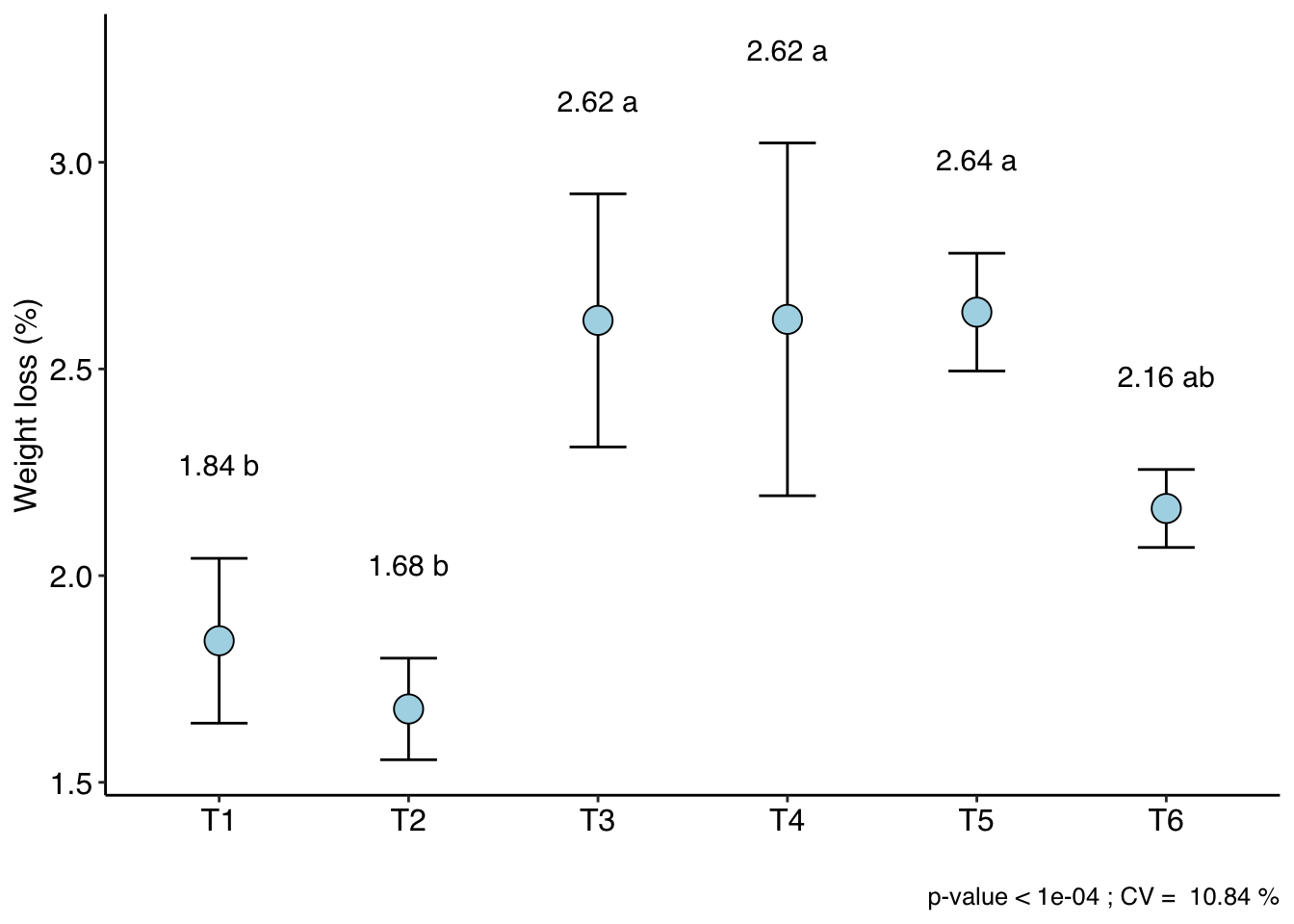
chart type: Graph type (columns, boxes or segments)

with(pomegranate, DIC(trat, WL, geom="point", ylab = "Weight loss (%)"))


-----------------------------------------------------------------
Normality of errors
-----------------------------------------------------------------
                         Method Statistic   p.value
 Shapiro-Wilk normality test(W) 0.9448293 0.2087967

As the calculated p-value is greater than the 5% significance level, hypothesis H0 is not rejected. Therefore, errors can be considered normal


-----------------------------------------------------------------
Homogeneity of Variances
-----------------------------------------------------------------
                              Method Statistic   p.value
 Bartlett test(Bartlett's K-squared)  8.568274 0.1275737

As the calculated p-value is greater than the 5% significance level,hypothesis H0 is not rejected. Therefore, the variances can be considered homogeneous


-----------------------------------------------------------------
Independence from errors
-----------------------------------------------------------------
                 Method Statistic   p.value
 Durbin-Watson test(DW)  2.104821 0.1924474

As the calculated p-value is greater than the 5% significance level, hypothesis H0 is not rejected. Therefore, errors can be considered independent


-----------------------------------------------------------------
Additional Information
-----------------------------------------------------------------

CV (%) =  10.84
MStrat/MST =  0.92
Mean =  2.2596
Median =  2.225
Possible outliers =  No discrepant point

-----------------------------------------------------------------
Analysis of Variance
-----------------------------------------------------------------
          Df   Sum Sq    Mean.Sq  F value        Pr(F)
Treatment  5 3.692121 0.73842417 12.31191 2.723541e-05
Residuals 18 1.079575 0.05997639

As the calculated p-value, it is less than the 5% significance level.The hypothesis H0 of equality of means is rejected. Therefore, at least two treatments differ



-----------------------------------------------------------------
Multiple Comparison Test: Tukey HSD
-----------------------------------------------------------------
     resp groups
T5 2.6375      a
T4 2.6200      a
T3 2.6175      a
T6 2.1625     ab
T1 1.8425      b
T2 1.6775      b

Step 4: Decode and Conclude

Interpret the CRD Results

Based on ANOVA p-values and multiple comparisons, identify significant differences in the response variable among treatments.

If differences are detected, pinpoint the treatment combinations responsible for those variations.

Consider the biological implications of observed differences and draw conclusions about treatment effects on the response variable.

By systematically following these steps, you’ll harness the analytical prowess of AgroR and CRD, unraveling the intricacies of your crop science experiments with precision and confidence.

Citation

BibTeX citation:

@online{santos2023,
  author = {Santos, Franklin},
  title = {Unveiling the {Power} of {Completely} {Randomized} {Design}
    {(CRD)} in {Crop} {Science} {Experiments}},
  date = {2023-10-24},
  url = {https://franklinsantos.com/posts/crd/},
  langid = {en}
}

For attribution, please cite this work as:

Santos, Franklin. 2023. “Unveiling the Power of Completely Randomized Design (CRD) in Crop Science Experiments.” October 24, 2023. https://franklinsantos.com/posts/crd/.